Training Support

A few years ago, portable GPS devices looked more like the clunky cellphones of the early 1990s. Today, athletes no longer need to drag along that much extra weight, as devices like the Garmin Forerunner 10 [1] have shrunk to the size of digital LED watches from the 1970s (Figure 1). These ultimate sports accessories log geographic coordinates during runs.

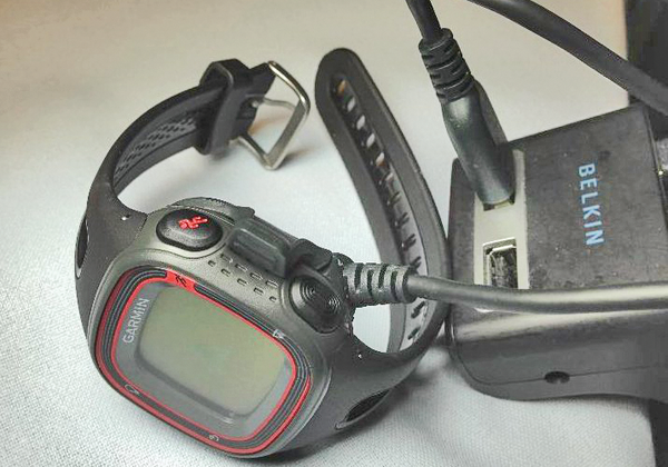
Figure 1: The wristwatch-sized GPS receiver logs the coordinates of points on the route traveled with timestamps.

Thus, runners can see how fast they are currently traveling and whether they need to speed up or slow down to achieve their own time goals. After completing all of this muscular activity, runners can then enjoy the experience of logging new speed records, viewing the running route on a map, reviewing the miles traveled, or marveling at an altitude profile of the route.

After plugging the Garmin 10 device into a USB port on my Ubuntu machine (Figure 1), the Linux kernel immediately detects the device as a storage unit and mounts the files stored on the device under /media/GARMIN. However, to do this, I did need a special adapter cable that clings to the GPS watch like a creature from the movie Alien and that came with the Garmin package. In the GARMIN/ACTIVITY directory, Linux users will find the FIT files in which the manufacturer stores motion activities in a proprietary binary format.

Athletes can upload these files to a newly created account on the Garmin website [2] and then view a presentation of the run data (Figure 2). The example shows an approximately five-mile route around Lake Merced – a lake near the Pacific Ocean just south of San Francisco  – which I ran for this Perl column in about 40 minutes.

Figure 2: On the Gamin website, athletes can upload their FIT data for a graphical display.

The graph shows total time, average time per mile (8:45 minutes), and elevation change (300 feet). If you prefer metric units, you can change to kilometers and meters on the website.

The Six-Second Cycle

The GPS device determines the runner's position approximately every six seconds with the help of earth-orbiting navigation satellites; it then stores the data points as geographical latitudes and longitudes and measures the current speed and distance traveled.

Unlike other GPS units, the Garmin 10 does not determine the current altitude above sea level during the run; apparently, this would require more expensive hardware to get right. But the Garmin website effortlessly fills this topographic gap in the movement profile based on the coordinates, using a server-side static elevation profile that probably knows the altitude of any inhabited part of the earth. Unless you are running up the stairs in a high rise, you will receive accurate altitude information for your run in this way.

Do It Yourself

Even the neatest website can be improved; some people want to remodel their data for seemingly esoteric purposes. Instead of painstakingly decrypting the proprietary format, you can pick up the Garmin SDK online [3]. Although the SDK does not define a Perl API, it does document all the data structures used in the log data.

On the basis of this information, developer Kiyokazu Suto built a Perl module [4] under a public domain-like license, but so far it has not been uploaded to CPAN. From the developer's website, you can download Garmin::FIT, which reads FIT files; Figure 3 shows an example of how the fitdump utility included with the module outputs the data.

Figure 3: The raw data read from the FIT format shows that the device determines its latitude and longitude, the current speed, and the distance traveled approximately every six seconds.

Despite the format having been disclosed, extracting the data from the binary blob proves to be a Sisyphean task. The Garmin::FIT module offers the print_all_fields() method, which I leveraged to hash up the dumper in Listing  1 [5]; it produces the output in Figure 3. To process the data, developers need to dig deeper and write their own functions.

Extracting from FIT

Listing 2 thus takes on the task of reshaping the FIT data and producing an easily readable YAML file. To do this, line 14 loads a FIT file passed in at the command line into the Garmin::FIT module. The goal of the subsequent procedure is to create a Perl array with the data from the record entries in the FIT file and then call the DumpFile() function from the YAML module to dump them as YAML data into a .yaml file of the same name.

To search the FIT data, line 19 calls the data_message_callback_by_name() method and sets up a callback that the FIT parser invokes for each entry found. The callback function message defined beginning in line 38 extracts the important values from the given parameters and puts them together to create a new data structure.

As Figure 4 shows, the current total run distance does not reside directly in the distance entry of the variable $v presented to the callback. Instead, the data structure $desc contains a number of values that the user must combine in mysterious ways to arrive at the desired result. To get the total distance, for example, the i_distance key in $desc contains an array index number (the number 4 in this case), which can be used to extract the desired total distance from the $v array as $v[4]. Then, fit2yaml combines this with the unit m for meters and determines the result with the Garmin::FIT value_cooked() method.

Figure 4: The Garmin format proves to be idiosyncratic. The distance, for example, is coded in $v[4].

The method still needs the value for a_distance (scaling and units) and the value for I_distance (validity scope) so that it can finally arrive at the desired value for the distance. Because the format can store all kinds of data in a tiny space, this method was most likely chosen to save space.

For simplicity's sake, Listing 2 does not attempt to handle all the supported data formats but focuses on the record entries with the run data sampled every six seconds. Other logged events, such as where and when the runner pressed the Start button, are ignored to limit the scope of the script.

Figure 5 shows the finished YAML data: a list of records that each contain a distance field (distance traveled from the start in kilometers), position_lat (latitude), position_long (longitude), speed (in meters per second), and timestamp (current time).

Figure 5: These entries show the Garmin GPS data in YAML format, as determined by the script in Listing 2.

Invisible Pacemaker

Once I have the YAML data, I can easily write applications in Perl and other languages that interpret the stored GPS data. One feature I really miss with my Garmin 10 (and that my previously used Garmin Forerunner 101 had) is the so-called Virtual Partner.

With this feature, runners can program in the speed of a virtual pacesetter, who runs at constant speed and crosses the finish line at precisely the expected time by definition. During the run, the GPS device indicates how far the virtual runner's legs have taken them. If the pacemaker is 100 yards ahead, I need to speed up, if it drops back, I can slow down, and if we are jogging together, I am sure to finish on time.

Listing 3 implements a function to compare two runs in a similar way for my new GPS device. It uses two FIT files converted into YAML format, reads the distance and timestamp entries, and draws a graph with the distances covered by the two runners at specific times. The x-axis shows the elapsed running time in seconds, and the y-axis visualizes the distance covered by the runners in meters.

Both FIT files were created during real runs. After my sporting excursion (Figure 2), I completed another training run on the same route. I wanted to find out whether a slightly slower pace in the first few miles would leave me feeling stronger for the final sprint and leave enough breathing room to manage a few hills in between (elevation difference about 300 feet).

The CPAN Imager::Plot module plots the data passed in as an array on the coordinate system and labels the axes nicely. The data_extract() function in line 59 expects a YAML file with the FIT data and returns an array. It contains x/y value pairs of stored combinations of timestamps and distances traveled.

Line 74 removes the unit, m for "meters," from the value for distance, leaving only the numeric value. The variable $base is set to the timestamp of the first entry, so that vrunner can later only add timestamps relative to this base point and append them to the resulting array.

Clockwork Horse

The green graph in Figure 6 shows the first, fast run; the red graph was created after the second, slower run. The comparison shows that I was unable to translate the power reserves gained by the slower starting pace into a faster second half. Once I'm in motion, I seem to run like clockwork – without anyone dangling a carrot in front of my nose, I seem to run no faster than necessary.

Figure 6: The laid-back jogger in red is steadily losing against the runner in flattering green, who is apparently pushing himself to the limit.