While I was working on hikefind, a command-line program that chooses a trail from a collection of GPX files with track points, for a recent issue [1], I got the idea of drawing the trail contours the program found in a terminal window. Unfortunately, a GPX file generated by an app such as Komoot or a Garmin tracker only contains geocoordinates as floating-point numbers. They refer to the points of the globe through which the trail passes (Figure 1).

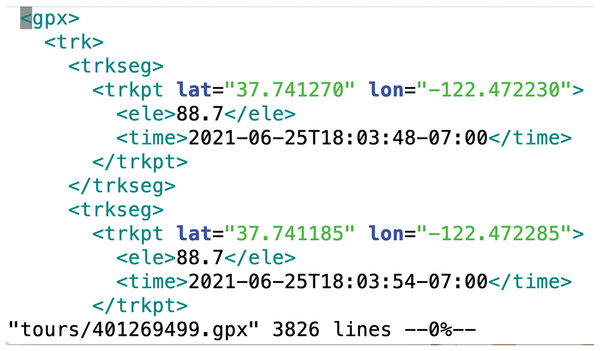Figure 1: Geocoordinates in a GPX file.

These geopoints on a spherical surface now need to be converted to a two-dimensional coordinate system so that they look as natural as possible on a flat map. This problem was solved centuries ago. Any map, whether paper or digital, is based on the genius idea of projecting geopoints on the globe, which are available as latitude and longitude values, onto an XY coordinate system on a plane.

Back to the Year 1569

As early as 1569, Gerhard Mercator, a cartographer from Flanders, set out to flatten the spherical data determined by early sea navigators. To do this, he simply projected the spherical surface of the Earth onto a cylinder wound around it (Figure 2). The outer layer of the cylinder, in turn, can be easily unrolled and viewed as a flat map. However, this projection (with a vertical winding cylinder) is only 100 percent correct at the equator and suffers from distortions to the north or south of it, until – finally – grotesquely inflated land masses appear in the polar regions.

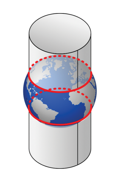Figure 2: A cylinder wrapped around the globe for the Mercator projection [2]. Wikipedia, CC BY-SA 4.0

But when it comes to drawing my trails in a terminal window, an even simpler mechanism will do the trick. The algorithm simply interprets the numerical degrees for longitude and latitude as values that increase linearly with the actual distance on the globe. In other words, the method interprets an area on the surface of a sphere constrained by longitude and latitude as a simple rectangle, even though the actual object is curved. This is not exactly accurate, of course, but it comes very close to the truth for relatively small areas in the context of the gigantic spherical radius of the Earth.

Minima and Maxima

For example, if a trail extends between longitudes -31.002 and -31.001 (longitudes west of the prime meridian have negative values), and the display terminal has a width of 80 characters, the linear projection maps the longitudes to integer X-values between 0 and 79 (Figure 3). The sample principle applies to latitudes and their projected Y-values.

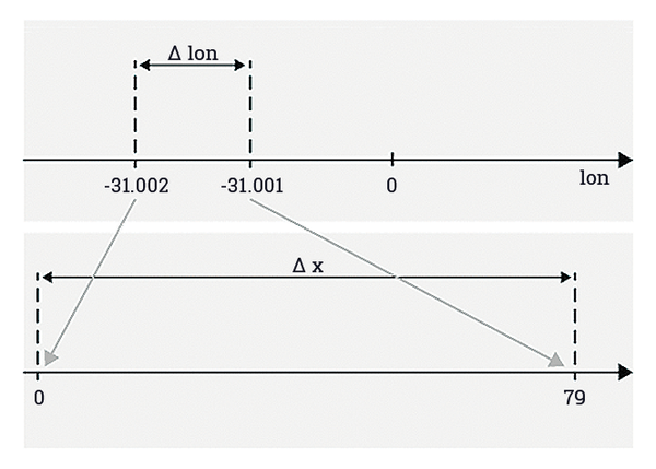Figure 3: The simple linear projection from longitude (lon) to X-values is good enough.

To do this, Listing 1 uses the projectSimple() function starting in line 28 to first determine the minimum and maximum values for the geographical latitude and longitude of all track points of the recorded trail as the latMin/latMax and lonMin/lonMax variables. During the first round of the for loop starting in line 33, the variable first is set to true, and the function initializes the overall min/max values found to the position of the first track point. In the following rounds, first is set to false, and the extremes only change if the current track point is outside the previously defined window.

Once the for loop is done with all the track points, lines 56 and 57 set the widths of these windows to latSpan and lonSpan. Given this maximum bandwidth, lines 59 and 60 compute the X- and Y-coordinates for the target coordinate system in the terminal window. To do this, they determine the distance of the current track points in the GPX data from the left or bottom edge of the window, divide this by the window width, and multiply the resulting floating-point value by the width of the target system.

This gives me the X- and Y-values from 0 to width-1 and height-1 in the target window, which is width characters wide and height characters high. Because the X-coordinates in the terminal window later run from left to right, but the Y-coordinates (especially in the GUI shown below) run from top to bottom, line 61 turns the Y-values on their heads.

Initially, the gpxPoints() function reads the data from the GPX file starting in line 11 in Listing 1 and conveniently provides it to the caller as an array slice of floating-point values. The gpx package from GitHub lends a hand in interpreting the GPX format here; it will be downloaded and included in the source code automatically later on when you compile the binary.

At the end of Listing 1 there is a cmdLineParse() function, which you need in the various main programs to analyze the command-line parameters, as submitted by users typing them in the shell.

On Screen!

The main program for easy plotting of the GPX data in a terminal (Listing 2) expects a GPX file with the XML-encoded geodata of a trail as an argument on the command line. It uses the gpxPoints() function from Listing 1 to extract the track points. Line 18 in Listing 2 calls the projectSimple() function from Listing 1 and passes both an array slice of GPX points and the dimensions of the current terminal, which are dynamically determined by the GitHub term package. The returned object is an array slice with the XY coordinates of the track points projected onto the flat terminal area.

To allow the line-by-line output starting in line 24 to quickly check whether the terminal cell in the current output contains the trail's track point, line 17 creates a map named isSet. It uses a row and column index to reference a Boolean value that is true for track points and false everywhere else. In a scripting language such as Python, this could be done easily with a two-dimensional hashmap or matrix. But doing this in Go is a Sisyphean task, because the program code needs to manually handle second-order memory management, which bloats the code disproportionately. This is why Listing 2 resorts to a trick and uses a one-dimensional map. The index here is the integer value y*width+x (i.e., the offset of the current element if you treat the cells along all the terminal rows as a continuous array).

The double for loop starting in line 24 then finally outputs the trail line-by-line on the terminal (Figure 4). To do this, the code first assumes that there isn't a track point for the coordinate currently being processed; this is why it sets the output string ch to a space character. But if the lookup in the isSet() map reveals that there indeed is a track point, it sets the string to an asterisk character *. Line 30 outputs the contents of the current cell and then moves on to the next round; it does this until it reaches the end of the current line and then moves on to the next line.

Figure 4: The trail on Komoot in a browser …

The usual three-card trick, shown in Listing 3, compiles the source files and links in the packages I referenced from GitHub. The result is a binary named gpx-plot, which expects the name of a GPX file, as shown in Figure 5, and then draws the track points from the file on standard output in the terminal.

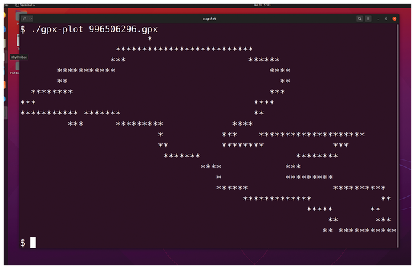Figure 5: … and on the terminal courtesy of gpx-plot.