
Request Spotify dossiers and evaluate them with Go and R
Streaming services such as Spotify or Apple Music dominate the music industry. Their extensive catalogs now cover the entire spectrum of consumable music. Relying on artificial intelligence, these services introduce users to new songs they'll probably like, as predicted by the services' algorithms. Traditional physical music media no longer stand a chance against this and gather dust on the shelves. Of course, this development also means that anonymous music consumption is a thing of the past, because streaming services keep precise records of who played what track, when, and for how long.
On request, Spotify will even hand over the acquired data (Figure 1). If you poke around a bit on their website, you'll find the buttons you need to press to request a copy of these files in Account | Privacy Settings, but Spotify takes their sweet time to respond. From the time of the request, it takes about a week for their archivist to retrieve the data from the files in the Spotify basement, compress them, and post them as a ZIP archive on the website for you to pick up. After receiving Spotify's email notification, you can then download the data for two weeks and poke around in it locally to your heart's content.
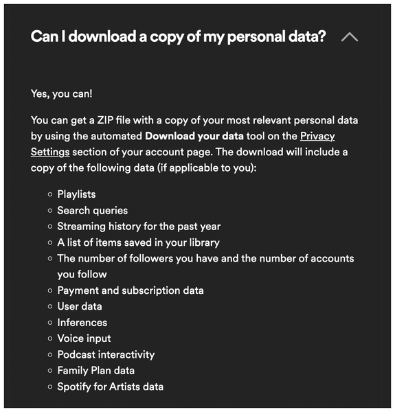 Figure 1: Spotify lets its users view the data it collected about them.
[...]
Buy this article as PDF
(incl. VAT)
Buy Linux Magazine
Subscribe to our Linux Newsletters
Find Linux and Open Source Jobs
Subscribe to our ADMIN Newsletters
Support Our Work
Linux Magazine content is made possible with support from readers like you. Please consider contributing when you’ve found an article to be beneficial.

News
-
Ubuntu Core 26 Offers Game-Changing Enterprise Features
Ubuntu Core 26 could be a game-changer for organizations looking for increased security and reliability.
-
AI Flooding the Linux Kernel Security Mailing List
AI is giving Linus Torvalds a headache, but not in the way you might think.
-
Top Priorities for Open Source Pros Seeking a New Job
Professional fulfillment tops the list, according to LPI report.
-
Container-Based Fedora Hummingbird Designed for Agent-First Builders
Fedora Hummingbird brings the same approach to the host OS as it does to containers to level up security.
-
Linux kernel Developers Considering a Kill Switch
With the rise of Linux vulnerabilities, the kernel developers are now considering adding a component that could help temporarily mitigate against them… in the form of a kill switch.
-
Fedora 44 Now Gaming Ready
The latest version of Fedora has been released with gaming support.
-
Manjaro 26.1 Preview Unveils New Features
The latest Manjaro 26.1 preview has been released with new desktop versions, a new kernel, and more.
-
Microsoft Issues Warning About Linux Vulnerability
The company behind Windows has released information about a flaw that affects millions of Linux systems.
-
Is AI Coming to Your Ubuntu Desktop?
According to the VP of Engineering at Canonical, AI could soon be added to the Ubuntu desktop distribution.
-
Framework Laptop 13 Pro Competes with the Best
Framework has released what might be considered the MacBook of Linux devices.