
Getting started with the R data analysis language
Data Cleanup
Data cleanup examples are difficult to generalize, because the actions you need to take heavily depend on the individual dataset. But there are a number of fairly common actions. For example, you might need to rename cryptically labeled columns. The recommended approach is to first standardize the designations. Then change the column names with the colnames() command. Then pass in the index of the column whose name you want to change in square brackets. The index of a particular column can also be found automatically (Listing 5, first line). If you do not want to overwrite the column caption of the original mtcars dataset, first copy the data to a new data frame with df <- mtcars.
Listing 5
Data Cleanup
> colnames(mtcars)[colnames(mtcars) == 'cyl'] <- 'Zylinder'
> without.zeros <- na.omit(mtcars)
> without.duplicates <- unique( mtcars )
If the records have empty fields, this can lead to errors. That's why it is a good idea to resolve this potential worry at the start of the cleanup. Depending on how often empty fields occur, you can either fill them with estimated values (imputation) or delete them. The command from the second line of Listing 5 removes all lines that contain at least one zero (also NaN or NA).
Records also often contain duplicates. If the duplicate is the result of a technical error in data retrieval or in the source system, you should first try to correct this error. R provides an easy way to clean up the dataset and assign the results to a new, clean data frame with the unique() command (Listing 5, last line).
Predictive Modeling
In reality, there are a variety of prediction models with a wide range of parameters that provide better or worse results depending on the requirements and data. For an example, I'll use a dataset for irises (the flowers) – one of the best-known datasets for machine learning examples.
As an algorithm, I use a decision tree to predict the iris species – given certain properties, for example, the length (Petal.Length) and width (Petal.Width) of the calyx. To do this, I first need to load the data, which already exists in an R library (Listing 6, line 1).
Listing 6
Prediction with Iris Data
01 > data(iris)
02 > n <- nrow(iris)
03 > n_train <- round(.70 * n)
04 > set.seed(101)
05 > train_indicise <- sample(1:n, n_train)
06 > iris_train <- iris[train_indicise, ]
07 > iris_test <- iris[-train_indicise, ]
08 > install.packages("rpart ")
09 > install.packages("rpart.plot")
10 > library(rpart)
11 > library(rpart.plot)
12 > iris_model <- rpart(formula = Species ~.,data = iris_train, method = "class")
13 > rpart.plot(iris_model, type=4)
The next thing to do is to split the data into training and test data. The training data is used to train the model, whereas the test data checks the predictions and evaluates how well the model works. You would typically use about 70 percent of the data for training and the remaining 30 percent for testing. To do this, first determine the length of the record using the nrow() function and multiply the number by 0.7 (Listing 6, lines 2 and 3). Then randomly select an appropriate amount of data (line 5).
I have set a seed of 101 for the random value selection in the example (line 4). If you set the same value for the seed, you will see identical random values. Following this, split the data into iris_train for training and iris_test for validation (lines 6 and 7).
After splitting the data, you can train and evaluate the decision tree model. To do this, you need the rpart library. rpart.plot visualizes the decision tree (lines 8 to 11). Next, generate the decision tree based on the training data. When doing so, pass in the Species column in order to predict which iris species you are looking at (line 12).
One advantage of the decision tree is that it is relatively easy to see which parameters the model refers to. rpart.plot lets you visualize and read the parameters (line 13). Figure 5 shows that the iris species is setosa if the Petal.Length is greater than 2.5. If the Petal.Length exceeds 2.5 and the Petal.Width is less than 1.7, then the species is probably versicolor. Otherwise, the virginica species is the most likely.
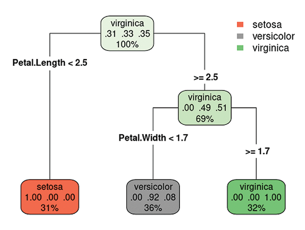 Figure 5: Visualizing the decision tree model with the iris data.
The next step in the analysis process is to find out how accurate the results are. To do this, you need to feed the model data that it hasn't seen before. The previously created test data is used for this purpose. Then use predict() to generate predictions based on the test data using the iris_model model (Listing 7, line 1).
Listing 7
Accuracy Estimation
01 > iris_pred <- predict(object = iris_model, newdata = iris_test, type = "class")
02 > install.packages("caret")
03 > library(caret)
04 > confusionMatrix(data = iris_pred, reference = iris_test$Species)
There are a variety of metrics for determining the quality of the model. The best known of these metrics is the confusion matrix. To compute a confusion matrix, first install the caret library (lines 2 and 3), which will give you enough time for an extensive coffee break even on a fast computer. Then evaluate the iris_pred data (line 4).
The statistics show that the model operates with an accuracy of 93 percent. The next step would probably be to optimize the algorithm or find a different algorithm that offers greater accuracy.
You can now also imagine how this algorithm could be applied to other areas. For example, you could use environmental climate data (humidity, temperature, etc.) as the input, combine it with information on the type and number of defects in a machine, and use the decision tree to determine the conditions under which the machine is likely to fail.
Importing Data
If you want to analyze your own data now, you just need to import the data into R to get started. R lets you import data from different sources.
To import data from a CSV file, first pass the file name (including the path if needed) to the read.table() function and optionally specify whether the file contains column names. You can also specify the separator character for the fields in the lines (Listing 8, first line).
Listing 8
Data Import
> df <- read.table("meine_datei.csv", header = FALSE, sep = ",")
> my_daten <- read_excel("my_excel-file.xlsx")
If the data takes the form of an Excel spreadsheet, you can also import it directly. To do this, install the readxl library and use read_excel() (second line) to import the data.
« Previous 1 2 3 4 Next »
Buy this article as PDF
(incl. VAT)
Buy Linux Magazine
US / Canada
UK / Australia
Subscribe to our Linux Newsletters
Find Linux and Open Source Jobs
Subscribe to our ADMIN Newsletters
Support Our Work
Linux Magazine content is made possible with support from readers like you. Please consider contributing when you’ve found an article to be beneficial.

News
-
Endless OS 6 has Arrived
After more than a year since the last update, the latest release of Endless OS is now available for general usage.
-
Fedora Asahi 40 Remix Available for Macs with Apple Silicon
If you've been anticipating KDE's Plasma 6 for your Apple Silicon-powered Mac, then you're in luck.
-
Red Hat Adds New Deployment Option for Enterprise Linux Platforms
Red Hat has re-imagined enterprise Linux for an AI future with Image Mode.
-
OSJH and LPI Release 2024 Open Source Pros Job Survey Results
See what open source professionals look for in a new role.
-
Proton 9.0-1 Released to Improve Gaming with Steam
The latest release of Proton 9 adds several improvements and fixes an issue that has been problematic for Linux users.
-
So Long Neofetch and Thanks for the Info
Today is a day that every Linux user who enjoys bragging about their system(s) will mourn, as Neofetch has come to an end.
-
Ubuntu 24.04 Comes with a “Flaw"
If you're thinking you might want to upgrade from your current Ubuntu release to the latest, there's something you might want to consider before doing so.
-
Canonical Releases Ubuntu 24.04
After a brief pause because of the XZ vulnerability, Ubuntu 24.04 is now available for install.
-
Linux Servers Targeted by Akira Ransomware
A group of bad actors who have already extorted $42 million have their sights set on the Linux platform.
-
TUXEDO Computers Unveils Linux Laptop Featuring AMD Ryzen CPU
This latest release is the first laptop to include the new CPU from Ryzen and Linux preinstalled.